Continue Pneumonia Classifier by moving to AWS SageMaker

In this post, we will continue Pneumonia Classifier practice by leveraging AWS managed AI service SageMaker. We will:

• Provision AWS Sagemaker AI domain and workspace.
• Run a JupiterLab to download, process, and upload chest X-ray dataset from Kaggle to S3 for SageMaker access.
• Use SageMaker Pre-built image classification algorithm, to define SageMaker Estimator to configure the SageMaker training job, including compute resources, training duration, and data input method.
• Count the number of training samples and set the hyperparameters, perform hyperparameter tuning to find the best configuration for the model.
• Launching the Hyperparameter Tuning Job.
• Using CloudWatch and SageMaker Train Job to monitor and troubleshoot.

In the AWS SageMaker AI JupiterLab

I will skip the dataset download as this task remains the same as what I did in the previous post.

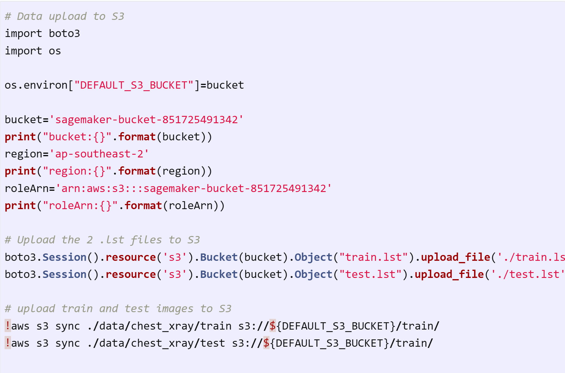
S3 will be the storage where SageMaker will access the dataset. Let's start from data upload.

Next step is to set up the SageMaker estimator to define the training job, including compute resources, training duration, and data input method. We will use the built-in algorithm for image classification.

# Set up SageMaker framework, execution_role and S3 location

import sagemaker
from sagemaker import image_uris
import boto3
from sagemaker import get_execution_role
sess=sagemaker.Session()

algorithm_image=image_uris.retrieve(
    region=boto3.Session().region_name,
    framework="image-classification",
    version="latest"
)

s3_output_location=f"s3://{bucket}/models/image_model"
print(algorithm_image)

role=get_execution_role()
print(role)

Set up the SageMaker estimator to define the training job. We will use the built-in algorithm for image classification with ml.g4dn.xlarge as spot GPU instance for job training.

# Set up SageMaker estimator
import sagemaker
img_classifier_model=sagemaker.estimator.Estimator(
    algorithm_image,
    role=role,
    instance_count=1,
    instance_type="ml.g4dn.xlarge",
    use_spot_instances=True,  # Enable spot instances
    max_run=432000,           # 5 days (432,000 seconds)
    max_wait=432000,          # Must be >= max_run
    volume_size=50,
    input_mode="File",
    output_path=s3_output_location,
    sagemaker_session=sess
)
print(img_classifier_model)

Setup the total number of labeled images to define epochs and batch size for training job.

# Define epochs and batch size
import glob 
count=0

for filepath in glob.glob('./data/chest_xray/train/*.jpeg'):
    count+=1
print(count)

count = 5216  # Example: Total training images
img_classifier_model.set_hyperparameters(
    image_shape='3,224,224',
    num_classes='2',  # As string
    use_pretrained_model='1',  # As string
    num_training_samples=str(count),  # As string
    augmentation_type='crop_color_transform',
    epochs='15',  # As string
    early_stopping='True',  # As string
    early_stopping_min_epochs='8',
    early_stopping_tolerance='0.0',
    early_stopping_patience='5',
    lr_scheduler_factor='0.1',
    lr_scheduler_step='8,10,12'
)

Perform hyperparameter tuning to find the best configuration for the model with metrics to evaluate model quality.

# Hyperparameter tuning
from sagemaker.tuner import CategoricalParameter,ContinuousParameter,HyperparameterTuner

hyperparameter_ranges={
    "learning_rate":ContinuousParameter(0.01,0.1),
    "mini_batch_size":CategoricalParameter([8,16,32]),
    "optimizer":CategoricalParameter(["sgd","adam"])
}

objective_metric_name="validation:accuracy"
objective_type="Maximize"
max_jobs=5
max_parallel_jobs=1

tuner=HyperparameterTuner(estimator=img_classifier_model,
                         objective_metric_name=objective_metric_name,
                         hyperparameter_ranges=hyperparameter_ranges,
                         objective_type=objective_type,
                         max_jobs=max_jobs,
                         max_parallel_jobs=max_parallel_jobs  
                         )

                         from sagemaker.session import TrainingInput

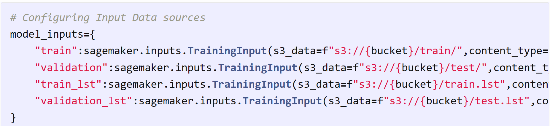
Configuring input data sources by specifying the S3 paths and content types for SageMaker training jobs.

Launching the Hyperparameter Tuning Job

# Start the hyperparameter tuning job with the specified inputs and configurations
import time 
job_name_prefix="classifier"
timestamp=time.strftime("-%Y-%m-%d-%H-%M-%S",time.gmtime())
job_name=job_name_prefix+timestamp

tuner.fit(inputs=model_inputs,job_name=job_name,logs=True)

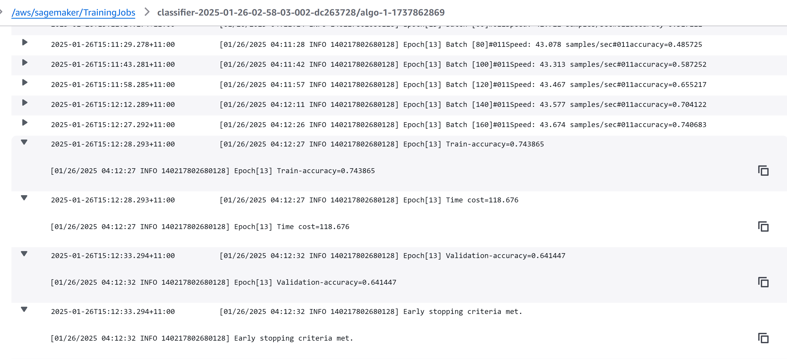
Monitor the tuning job in the AWS SageMaker console to track progress.

Go to CloudWatch SageMaker log group to see detailed logs of the training job.

Key Factors Influencing Runtime

Total training runtime and performance influenced by Tesla T4 GPU instance ml.g4dn.xlarge and the total 15 epochs of 5216 training samples.

Tesla T4 typically takes ~0.5-1 second per batch for tasks of this complexity, so the total Hyperparameter Tuning Time: 5 jobs × 41 minutes per job = 205 minutes (3.4 hours).

Increase max_parallel_jobs to run multiple jobs concurrently (e.g., max_parallel_jobs=2 would cut the runtime in half). Use a more powerful instance (e.g., ml.p3.2xlarge with a V100 GPU for faster training).

Deploy the trained model to validate prediction

Creates a SageMaker model object using the trained model's artifacts (model_data) and algorithm container (image_uri). Deploys the model as a SageMaker endpoint using the deploy() method. Using an instance type (ml.m4.xlarge) to offer endpoint for real-time inference.

model = sagemaker.model.Model(
    image_uri=algorithm_image,
    model_data='s3://sagemaker-bucket-851725491342/models/image_model/classifier-2025-01-26-02-58-03-001-a577816e/output/model.tar.gz',
    role=role
)
endpoint_name = 'zack-super-cool-endpoint'

deployment = model.deploy(
    initial_instance_count=1,
    instance_type='ml.m4.xlarge',
    endpoint_name=endpoint_name
)

Setup and test the endpoint for real-time prediction. Send a testing payload in binary mode to the endpoint for prediction.

from sagemaker.predictor import Predictor
predictor = Predictor("zack-super-cool-endpoint")

from sagemaker.serializers import IdentitySerializer
import base64

file_name = 'data/chest_xray/val/val_normal0.jpeg'
predictor.serializer = IdentitySerializer("image/jpeg")

with open(file_name, "rb") as f:
    payload = f.read()
inference = predictor.predict(data=payload)
print(inference)

Output:
b'[0.8592441082997322, 0.14075589179992676]'

print(inference[1])

Output:
48

Run a batch prediction and evaluate the matrix. Now let's loop through all images in the validation dataset, send each image to the endpoint for prediction, collect predictions for all validation images to evaluate the model's overall performance, and print the classification report.

import glob
import json
import numpy as np

file_path = 'data/chest_xray/val/*.jpeg'
files = glob.glob(file_path)

y_true = []
y_pred = []

def make_pred():
    for file in files:
        if "normal" in file:
            with open(file, "rb") as f:
                payload = f.read()
                inference = predictor.predict(data=payload).decode("utf-8")
                result = json.loads(inference)
                predicted_class = np.argmax(result)
                y_true.append(0)  # Normal class
                y_pred.append(predicted_class)
        elif "pneumonia" in file:
            with open(file, "rb") as f:
                payload = f.read()
                inference = predictor.predict(data=payload).decode("utf-8")
                result = json.loads(inference)
                predicted_class = np.argmax(result)
                y_true.append(1)  # Pneumonia class
                y_pred.append(predicted_class)

make_pred()
print(y_true)
print(y_pred)

Output:
[0, 1, 0, 1, 0, 1, 0, 1, 0, 1, 1, 0, 1, 0, 1, 0,]
[0, 1, 0, 1, 0, 1, 1, 1, 0, 1, 1, 1, 1, 0, 1, 0,]

# Evaluate the metrics

from sklearn.metrics import confusion_matrix
confusion_matrix(y_true, y_pred)

Output:
array([[6, 2],
       [0, 8]])    

# print classification report
from sklearn.metrics import classification_report
print(classification_report(y_true, y_pred))

Output:

              precision    recall  f1-score   support

           0       1.00      0.75      0.86         8
           1       0.80      1.00      0.89         8

    accuracy                           0.88        16
   macro avg       0.90      0.88      0.87        16
weighted avg       0.90      0.88      0.87        16

Result Analysis

The classification report shows the following metrics:

Class	Precision	Recall	F1-Score	Support
0	1.00	0.75	0.86	8
1	0.80	1.00	0.89	8

Accuracy: 0.88 (88%)

Macro Avg: Precision = 0.90, Recall = 0.88, F1-Score = 0.87

Weighted Avg: Precision = 0.90, Recall = 0.88, F1-Score = 0.87

The confusion matrix is:

	Predicted 0	Predicted 1
Actual 0	6	2
Actual 1	0	8

True Positives (TP): 8 (correctly predicted pneumonia)

True Negatives (TN): 6 (correctly predicted normal)

False Positives (FP): 2 (normal misclassified as pneumonia)

False Negatives (FN): 0 (pneumonia misclassified as normal)

Conclusion

• Move image classification model to cloud ML service using AWS SageMaker, integrated with AWS services (IAM, S3, SageMaker, CloudWatch) for data storage and model deployment and monitoring.
• Set up a cloud-based real-time image prediction endpoint for the trained model.
• Test the endpoint with an individual input image to confirm functionality.
• Run predictions on a validation dataset to evaluate model accuracy and robustness.
• Use confusion matrices and classification reports to assess the quality of predictions and identify areas for improvement.